Loop and domain calling

This notebook demonstrates how to identify chromatin loops and TADs from the seqFISH+ dataset from Takei et al, 2021. The 25Kb subset used here can be downloaded from the 4DN data portal with file IDs: 4DNFIHF3JCBY (biological replicate 1) and 4DNFIQXONUUH (biological replicate 2).

import matplotlib.pyplot as plt
import arcfish as af

Loading FOF_CT-core file

arcfish.pp.FOF_CT_Loader is the base class to read in FOF_CT files. The input can be a string, a list, or a dictionary like here. It can also read in other FOF_CT files other than FOF_CT-core (check api documentation here).

For FOF_CT-core files, loader.chr_ids show a list of available chromosomes.

loader = af.pp.FOF_CT_Loader({
    "rep1": "4DNFIHF3JCBY.csv", "rep2": "4DNFIQXONUUH.csv"
}, nm_ratio={c: 1000 for c in "XYZ"})
loader.chr_ids

array(['chr1', 'chr2', 'chr3', 'chr4', 'chr5', 'chr6', 'chr7', 'chr8',
       'chr9', 'chr10', 'chr11', 'chr12', 'chr13', 'chr14', 'chr15',
       'chr16', 'chr17', 'chr18', 'chr19', 'chrX'], dtype=object)

The create_adata function creates an AnnData object for a specific chromosome with the following fields:

1. n_obs: the number of chromatin traces

2. n_vars: the number of imaging loci

3. X, Y, and Z: 3D coordinates

4. Chrom_Start and Chrom_End: 1D genomic location of each locus

5. Chrom: chromosome number (“chr6” in this case)

adata = loader.create_adata("chr6")
adata

AnnData object with n_obs × n_vars = 921 × 60
    var: 'Chrom_Start', 'Chrom_End'
    uns: 'Chrom'
    layers: 'X', 'Y', 'Z'

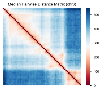
We can calculate the median pairwise distance matrix and visualize it using af.pp.median_pdist and af.pl.pairwise_heatmap.

af.pp.median_pdist(adata, inplace=True)
adata

AnnData object with n_obs × n_vars = 921 × 60
    var: 'Chrom_Start', 'Chrom_End'
    uns: 'Chrom'
    layers: 'X', 'Y', 'Z'
    varp: 'med_dist'

fig, ax = plt.subplots(figsize=(4, 3))
af.pl.pairwise_heatmap(adata.varp["med_dist"], ax=ax, cmap="RdBu",
                       title="Median Pairwise Distance Matrix (chr6)")

Loop calling

First we filter and normalize the data. This appends ‘med_dist’, ‘raw_var_X’, ‘raw_var_Y’, ‘raw_var_Z’, ‘count_X’, ‘count_Y’, ‘count_Z’, ‘var_X’, ‘var_Y’, ‘var_Z’ to the anndata object, where var_* are the axis variance matrices.

af.pp.filter_normalize(adata)
adata

AnnData object with n_obs × n_vars = 921 × 60
    var: 'Chrom_Start', 'Chrom_End'
    uns: 'Chrom'
    layers: 'X', 'Y', 'Z'
    varp: 'med_dist', 'raw_var_X', 'raw_var_Y', 'raw_var_Z', 'count_X', 'count_Y', 'count_Z', 'var_X', 'var_Y', 'var_Z'

Create a LoopCaller object with an FDR cutoff of 0.1. The call_loops() method returns a dictionary containing the analysis results.

caller = af.tl.LoopCaller(fdr_cutoff=0.1)
loop_result = caller.call_loops(adata)
loop_result.keys()

dict_keys(['axis_stat', 'axis_pval', 'stat', 'pval', 'fdr', 'candidate', 'label', 'summit', 'final'])

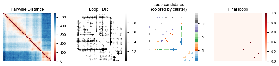
Now we create four heatmaps to visualize the loop calling process: the original distance matrix, FDR values, loop candidates grouped by clusters, and the final loop calls.

fig, axes = plt.subplots(1, 4, figsize=(9, 2))
af.pl.pairwise_heatmap(adata.varp["med_dist"], ax=axes[0], cmap="RdBu",
                       title="Pairwise Distance")
af.pl.pairwise_heatmap(loop_result["fdr"], ax=axes[1], cmap="Greys_r",
                       title="Loop FDR")
af.pl.pairwise_heatmap(loop_result["label"], ax=axes[2], cmap="tab20c",
                       title="Loop candidates\n(colored by cluster)")
af.pl.pairwise_heatmap(loop_result["final"], ax=axes[3], cmap="Reds",
                       title="Final loops")

Convert the loop results to BEDPE format using the to_bedpe() method, then filter for final loops and display the first few rows.

bedpe = caller.to_bedpe(loop_result, adata)
bedpe[bedpe["final"]].head()

	c1	s1	e1	c2	s2	e2	stat	pval	fdr	candidate	label	summit	final
1502	chr6	50300000	50325000	chr6	50525000	50550000	7.145024e+09	4.454981e-11	6.058774e-08	True	1.0	True	True
1729	chr6	50675000	50700000	chr6	50800000	50825000	1.741511e+06	1.827780e-07	6.214450e-05	True	8.0	True	True

TAD calling

Create a TADCaller object with FDR cutoff 0.1 and run call_tads() on the data. This returns a DataFrame with the TAD calling results.

Note here the data is already filtered and normalized. If the data is not preprocessed yet, run filter_normalize first.

caller = af.tl.TADCaller(fdr_cutoff=0.1)
tad_result = caller.call_tads(adata)
tad_result.head()

	c1	Chrom_Start	Chrom_End	stat_x	stat_y	stat_z	pval_x	pval_y	pval_z	stat	stat_prox	pval	fdr	fdr_peak	raw_peak	peak
0	chr6	49375000	49400000	NaN	NaN	NaN	NaN	NaN	NaN	NaN	NaN	NaN	NaN	False	False	False
1	chr6	49400000	49425000	NaN	NaN	NaN	NaN	NaN	NaN	NaN	NaN	NaN	NaN	False	False	False
2	chr6	49450000	49475000	0.976542	0.986278	0.932193	0.253538	3.494223e-01	2.560919e-02	4.802816e+00	0.018384	6.534212e-02	1.829579e-01	False	False	False
3	chr6	49475000	49500000	0.959849	0.917475	0.909965	0.086188	2.053673e-03	9.127656e-04	1.714311e+02	0.036911	1.856759e-03	8.664876e-03	True	False	False
4	chr6	49500000	49525000	0.889484	0.811094	0.861914	0.000053	2.063632e-12	4.926662e-07	4.873805e+10	0.078701	6.530998e-12	6.095598e-11	True	True	True

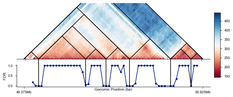
Visualize the TAD boundaries using triangle_domain_boundary(), which creates a triangle plot showing the domain structure.

fig = plt.figure(figsize=(7, 2.8))
ax, cbar, cax = af.pl.triangle_domain_boundary(adata, caller, fig=fig)

Convert the TAD results to BEDPE format and display the first few rows.

caller.to_bedpe(tad_result).head()

	c1	s1	e1	c2	s2	e2	stat1	stat2	level	idx1	idx2
0	chr6	49375000	49400000	chr6	49500000	49525000	NaN	4.873805e+10	0	0	4
1	chr6	49500000	49525000	chr6	49900000	49925000	4.873805e+10	2.508111e+01	0	4	20
2	chr6	49900000	49925000	chr6	50075000	50100000	2.508111e+01	1.021685e+08	0	20	27
3	chr6	50075000	50100000	chr6	50275000	50300000	1.021685e+08	5.160219e+15	0	27	35
4	chr6	50275000	50300000	chr6	50625000	50650000	5.160219e+15	1.633124e+16	0	35	48